How to Build a Replenishment Strategy for CPG Brands

Your purchase order is ready, but the allocation tab still doesn't balance. Amazon needs inventory, a retailer has a promotion coming, and your DTC warehouse is holding slow-moving stock you can't turn into cash quickly enough. Buying more might solve availability while making working capital worse.

A useful replenishment strategy answers two different questions: when to buy, and where the next available unit should go. Set those decisions at SKU, channel, and fulfillment-node level. Then judge the result by contribution, service, and cash, not by whether every channel carries the same days of cover.

How to Build Your Replenishment Strategy in Six Steps

RedDog's structured approach starts with Foundation, meaning clean data and SKU segmentation, moves into Optimization, meaning tuned forecasts and allocation rules, and reaches Amplification when additional channels can support the economics.

Build the operating sequence

1. Clean the transaction history. Start with a working dataset of 52 weeks of sales, inventory, and receipts by SKU, channel, and location. Reconcile duplicate orders, missing receipts, stockout periods, and inventory adjustments before treating shipped units as unconstrained demand.
2. Segment products using an ABC-XYZ grid. Rank ABC by contribution dollars and velocity, then use XYZ to distinguish stable demand from intermittent demand. Give high-value, predictable A/X products tight control; give C/Z products lower inventory commitments and explicit exception rules, rather than buying generous cover for erratic sellers.
3. Assign a forecast method to each segment. Use a simple baseline where demand is steady and a promotion-aware method where discounts change ordering behavior. Keep channel forecasts separate so a wholesale shipment doesn't inflate the Amazon baseline.
4. Measure the supplier lane, not just the supplier's promise. Record elapsed time from purchase-order release until inventory becomes sellable at the intended node, including production, transit, receiving, and check-in. Calculate both the average and the spread.
5. Set safety stock, reorder points, and allocation rules. Calculate the buffer for each SKU-channel pair, then check the resulting purchase against shelf life, minimum orders, case packs, and available cash. Decide which commitments receive inventory first before a shortage forces an improvised decision.
6. Put reviews on the calendar and exceptions in an alert queue. A practical starting cadence is weekly for A items, biweekly for B items, and monthly for C items, with immediate review whenever days of cover fall below replenishment lead time. Assign someone who can approve a purchase or change an allocation.

Use the process map as an orientation, while keeping the detailed review cadence appropriate to each segment.

Keep the system proportional

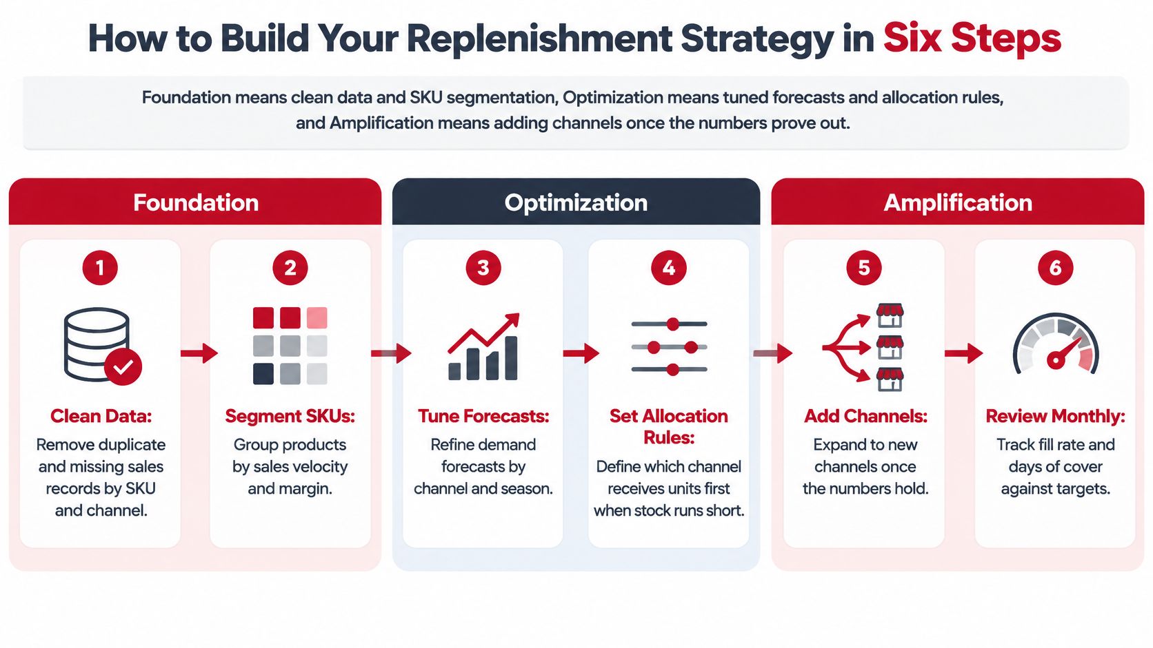
For an illustrative brand with about 20 SKUs, one controlled spreadsheet can support this workflow. At 200 or more SKUs, evaluate a planning tool with channel-level views against the time spent reconciling files and correcting mistakes.

The order matters. Safety stock calculated from uncleaned receipts produces precise-looking wrong numbers, and automation only repeats those errors faster.

Reorder Point and Safety Stock Formulas With Worked Numbers

Consider a hypothetical SKU selling 40 units daily, with a 21-day average lead time, 12 units of daily demand standard deviation, and 3.5 days of lead-time standard deviation. Its calculated reorder point is approximately 1,088 units. The important finding isn't the total, it's how much of the buffer comes from delivery uncertainty.

Calculate the inputs consistently

For this worked example, calculate average daily demand from 56 days of cleaned sales. Include zero-sales days when the item was available, but flag stockout days separately because zero shipments don't necessarily mean zero demand.

Calculate demand standard deviation from those daily observations. For lead time, use the last six purchase orders, measured through the date stock became sellable at the destination, not the supplier's dispatch date.

Replenishment formulas with a worked example

Under the normal approximation, use z = 1.65 for an illustrative 95% cycle-service target. Cycle service means the probability of avoiding a stockout during a replenishment cycle, not the percentage of customer units fulfilled.

The safety-stock calculation is:

1.65 × √[(21 × 12²) + (40² × 3.5²)] ≈ 248 units

This formula assumes demand and lead time are independent. If supplier delays coincide with peak demand, backtest the calculation against actual cycles rather than trusting the approximation alone.

Practical rule: Investigate lead-time variation before paying for more inventory to cover supposed demand uncertainty.

Separate the trigger from the purchase quantity

Buffering for demand alone gives 1.65 × 12 × √21 ≈ 91 units. Including lead-time variability raises the buffer to about 248 units, so the demand-only approach undercovers this example by approximately 63%. That demonstrates why lead-time uncertainty can dominate safety stock, not that it always will.

The reorder point is 40 × 21 + 248 = 1,088 units. Compare that threshold with inventory position, meaning usable on-hand stock plus reliable open inbound, less committed demand, so you don't duplicate purchases already underway.

An illustrative fixed order covering 45 days requires 1,800 units, exactly 75 cases of 24. That quantity still needs a cash and shelf-life check.

Reject three shortcuts: using a 7-day promotional average, treating returns or unfulfilled orders as shipped sales, and substituting quoted lead time for actual sellable dates.

Forecasting Methods Matched to Each SKU Segment

Choose the method that fits the available history, not the method with the most settings. A forecast earns its place by supporting better purchasing decisions on unseen periods. A complex model fitted to contaminated sales history won't rescue the replenishment plan.

Match complexity to the demand pattern

For a stable A item without promotions, test a moving average over 4 to 8 weeks as a planning candidate. It's transparent and easy to maintain, but it reacts late when demand changes direction. Test whether a 2-to-4-week lag would create an unacceptable purchasing delay rather than assuming the baseline updates fast enough.

A seasonal index needs repeated seasonal cycles. Use two full years as a practical minimum test dataset, and separate Amazon promotion weeks from ordinary demand before estimating seasonal effects. A shifted promotion calendar can otherwise look like a change in seasonality.

For growing products with recurring seasonal patterns, test Holt-Winters exponential smoothing. Constrain the smoothing parameters and validate the result so an isolated spike doesn't reset the purchasing baseline.

For launches, an illustrative approach uses the first 90 days of a comparable product. Match distribution, price, pack size, and advertising support before borrowing its curve. The analog choice often matters more than the calculation.

For marketplace-specific considerations, the inventory guidance from Online Brand Growth provides additional context. Use the inventory forecasting methods guide when comparing baseline approaches across a wider assortment.

Let the holdout decide

A workable test reserves the last 13 weeks, compares each candidate's bias and error by SKU, and selects the strongest practical result. Give persistent bias more attention than a small improvement in average error: sustained overforecasting commits cash, while sustained underforecasting leaves listings unavailable and orders unfilled.

Allow buyer overrides for confirmed distribution gains, retailer orders, or known events, but log the reason and compare the override with actual demand. As a starting operating policy, refresh A-item models monthly and the remainder quarterly, with event-driven changes between reviews.

Lead-Time Lanes and Supplier Buffers That Hold Up

The supplier quotes production time. Your customer needs sellable inventory. Between those points sit freight booking, port dwell, customs, warehouse appointments, and marketplace receiving, none of which disappears because a purchase order says the goods are ready.

Measure the full lane before deciding how much protection to buy. The following ranges are illustrative planning assumptions, not carrier commitments or published transit benchmarks; replace them with your own records.

Typical lead times and buffer days by sourcing lane

Fix the lane before enlarging the buffer

Start with six to ten completed POs as a working sample, then expand the history as records accumulate. Separate recurring delays from exceptional disruptions, and don't delete late receipts just because they make the supplier look unreliable.

Single-source packaging needs explicit contingency planning. A finished-goods buffer won't solve an unavailable closure indefinitely, and an ingredient MOQ can force cash commitments well beyond the finished-product order.

Supplier agreements should address capacity reservations, component ownership, and payment timing. The supplier relationship management guide is useful for structuring those conversations; for teams automating receipt-history analysis, Faberwork LLC's discussion of data-driven logistics improvements offers a technical starting point.

Price the rescue shipment

Assume air freight adds $1.80 per unit, contribution before that premium is $1.89, and demand is 40 units daily. Each otherwise unrecoverable stockout day costs $75.60 in contribution, while expediting 300 units costs $540.

The premium breaks even only if it prevents more than approximately 7.14 stockout days. Those units cover just 7.5 days of demand, so the direct financial case is narrow. Rank recovery, retailer commitments, or customer retention may justify acting earlier, but don't treat those benefits as guaranteed revenue.

Allocating Scarce Units Across Channels by Contribution

In the hypothetical comparison below, wholesale contributes $2.35 per unit, versus $0.67 for DTC, despite a much lower selling price. Wholesale isn't the highest-contribution option overall: Amazon FBM and Walmart WFS each reach $2.44 under these assumptions. That distinction matters when inventory is constrained.

The decision is which SKU-channel pair receives units, not just how many units to purchase. Availability matters to shoppers: the SPAR shopper survey document reports that 74% of surveyed shoppers identified product availability as their top in-store priority, while 73% cited out-of-stocks as a major barrier.

Use the allocation visual to frame the decision, then apply the actual contribution ledger rather than a channel label.

Compare contribution on the same basis

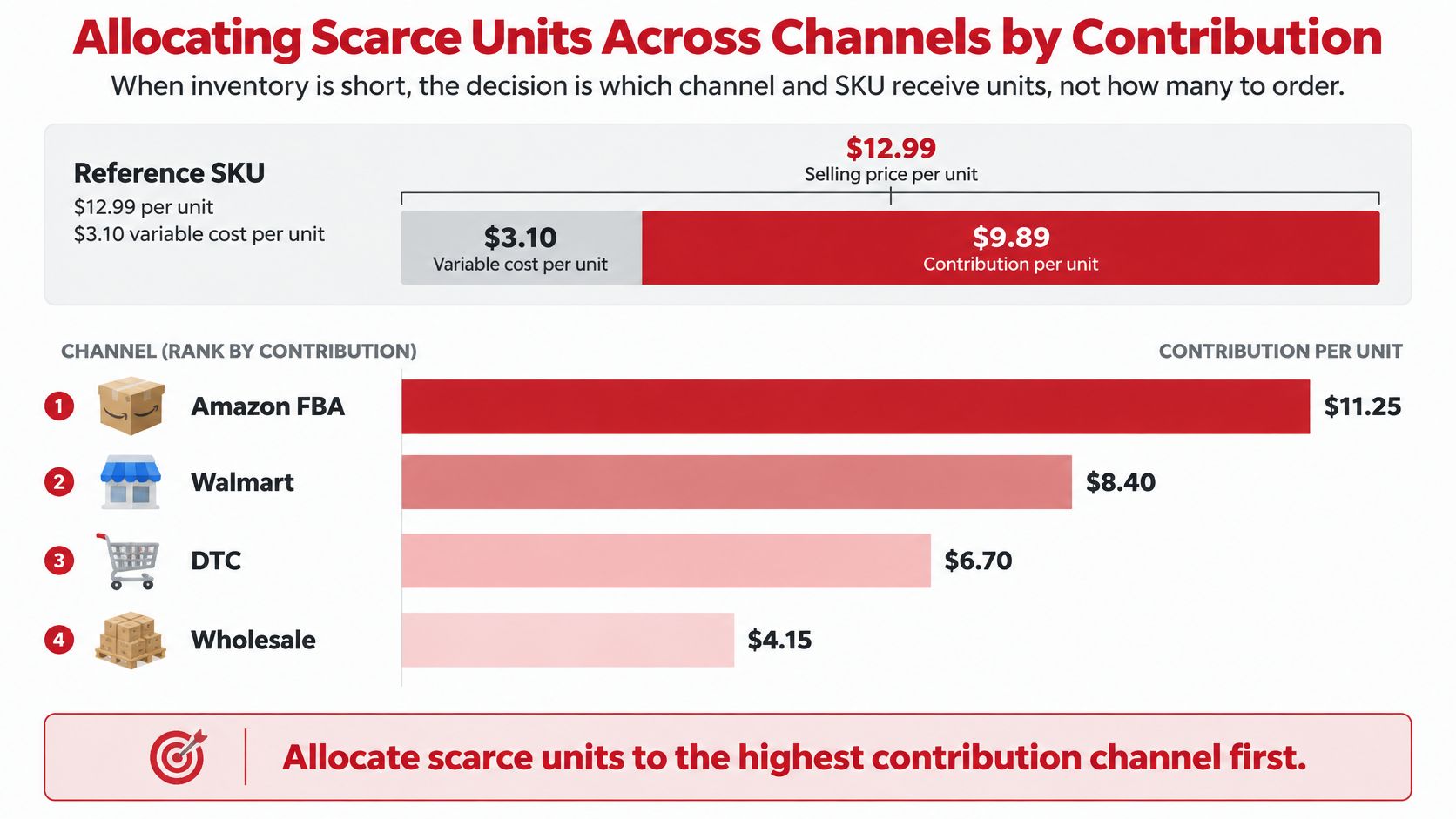
Every amount below is an illustrative assumption, not a current Amazon or Walmart fee quote. Check the SKU's size tier, shipping weight, fulfillment method, discounts, and current account charges before using the model.

Contribution per unit by channel for one sample SKU ($12.99 price, $3.10 COGS)

Use consistent treatment of returns, freight, payment fees, and deductions. The contribution margin calculation guide helps establish that common basis.

For the hypothetical FBA row, contribution before advertising is $4.49, producing a break-even advertising cost of sales of approximately 34.6%, before fixed overhead. That isn't a target: spending at break-even leaves nothing from those sales to fund overhead or profit.

Apply floors before discretionary ranking

Rank discretionary allocations using contribution per unit × expected daily velocity, then account for contractual commitments, substitution options, and replenishment timing. Treat the product as daily contribution potential, not a complete optimization formula. A fast channel can deserve inventory even when another channel earns more on each unit.

A channel floor protects a specific obligation or recovery risk. It shouldn't become an untouchable stockpile.

Suppose 800 units arrive, Amazon sells 40 daily, and a 400-unit wholesale order is due in 10 days. Reserve wholesale's committed quantity first, allocate an Amazon floor of 200 units, and allocate the remaining 200 units to DTC only if confirmed DTC commitments or its near-term floor require them.

Without that DTC requirement, sending the remainder there contradicts the contribution ranking. Floors are constraints, not permission to ignore economics, and Amazon's floor needs another inbound plan before it runs out.

For additional channel-allocation context, use the accompanying video.

Channel Rules for Amazon, Walmart, DTC and Wholesale

Applying one replenishment cadence everywhere is a common operational mistake. Amazon availability, a Walmart inbound appointment, a DTC reorder reminder, and a wholesale promotion require different decisions, even when they draw from the same production run.

Marketplace inventory also has a receiving stage. Stock in transit or awaiting check-in isn't necessarily available for customers to buy.

Channel triggers, constraints and failure modes

Separate platform rules from customer consumption

For FBA, compare expected depletion with realistic receiving availability and monitor inventory age. Verify current aged-inventory charges in the account's applicable fee schedule rather than hard-coding a universal threshold.

With FBM, the buffer sits in your warehouse, where storage, labor, and carrier execution remain your responsibility. For WFS, use its own inbound requirements; distinguish marketplace fulfillment requirements from Walmart wholesale OTIF obligations instead of assuming every program carries identical penalties.

DTC needs a consumption model, not just a subscription count. SmartCommerce's online trends report found that subscription usage declined from 37% to 29% year over year. That finding doesn't establish an individual brand's churn rate, but it challenges the assumption that fixed auto-delivery equals durable demand.

Use purchase intervals, pack size, seasonality, and promotion response to trigger predictive reminders. Reserve subscriptions for genuinely repetitive consumption and offer pause, skip, and frequency adjustments. Customers switching between DTC and marketplaces can otherwise look like lost demand in one forecast and unexpected demand in another.

For wholesale, validate the retailer's receiving calendar and promotional requirements before promising inventory. Teams coordinating case packs and customer commitments can explore wholesale stock management from UI Lib when assessing workflow options.

Watch the cost of fragmentation

Splitting inventory across channels reduces the opportunity to share one buffer. Each isolated location may need protection, while transfers add freight, handling, and time.

Risk to price explicitly: Inventory ownership doesn't mean inventory availability. Units in the wrong node can coexist with a customer-facing stockout.

The channel nobody forecasts can create the largest surprise. Include distributor orders, samples, replacements, and retailer promotions in the inventory plan, even when another team owns the relationship.

Confirm the Rollout Before Your Next Purchase Order

A purchase order released against unreconciled transactions locks cash into the wrong units. Before releasing the next PO, confirm that transaction history is reconciled, every supplier lane has a measured PO-to-sellable lead time, and each SKU-channel pair has approved purchasing settings. Name the channel owner and keep a live override log with the decision, reason, approver, and expiry condition.

Run the checklist as a release gate. The order stays blocked until every line passes.

Prepare the working files

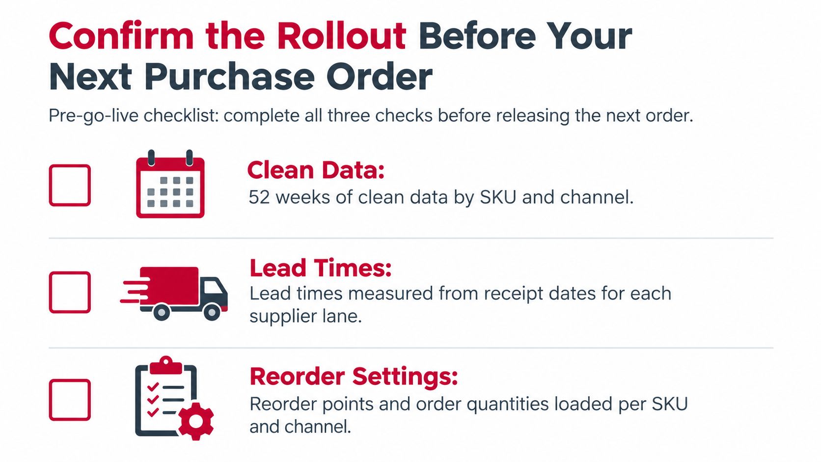
Build three connected templates before go-live:

• Channel reorder sheet. Include SKU, daily demand, lead time, safety stock, reorder point, usable inventory position, case pack, and cover target.
• Allocation sheet. Show available units, committed orders, channel floors, contribution-per-unit ranking, and the next expected sellable receipt. When a lane slips and units run short, this sheet decides which channel keeps its floor and which one waits for the next receipt.
• Bias tracker. Compare forecast with actual demand by segment, separating baseline performance from promotions and manual overrides.

Lock formula cells and document data-refresh ownership. A shared Excel workbook or Google Sheet is workable when everyone uses the same definitions and updates the same version.

Set operating tolerances

For an illustrative rollout, start with these internal targets, then adjust them to shelf life, service commitments, and cash constraints:

• Days of cover. Keep each channel within 5 days of its approved target.
• Forecast bias. Investigate segment bias outside plus or minus 10%.
• A-item availability. Target stockout days below 3% of selling days.
• Retailer service. Compare fill rate and OTIF with each account's actual contractual target.
• Inventory exposure. Review aged units, storage charges, and cash committed against plan.
• Inbound execution. Compare actual PO-to-sellable time with the planning input. A widening gap on a lane means its safety stock input is stale, since lead-time variability drives most of the buffer that lane carries.

Keep the segment-based review calendar, and reassess supplier variability and the allocation floors protecting high-contribution channels quarterly as an initial operating policy. Escalate material changes immediately rather than waiting for the scheduled review.

A replenishment strategy is ready to operate when the buyer can explain why the order exists, finance can see the cash commitment, and each channel owner knows what happens if the shipment arrives late.

Reddog Consulting Group offers CPG operators support with margin analysis, marketplace performance, and replenishment planning. Visit Reddog Consulting Group to book a strategy call on your reorder points, channel allocation, and contribution margins before your next purchase order.